Overview

Clustering high-dimensional categorical data poses unique challenges, particularly when traditional techniques struggle with the large number of features. While dimensionality reduction methods such as Principal Component Analysis (PCA) are commonly used to facilitate clustering, they are not inherently designed for categorical data, making their application less effective in this context.

To address these limitations, I employed an autoencoder framework to reduce the dimensionality of the dataset while preserving its key features. The autoencoder’s latent space, composed of continuous variables, offers a convenient representation for clustering algorithms, significantly improving their performance compared to directly clustering categorical data.

Autoencoder Design and Testing

To identify the optimal autoencoder architecture for this project, I systematically tested several configurations and evaluated their performance based on:

• Reconstruction Loss: Comparing the accuracy of the reconstructed data to the original data.

• Clustering Results: Analyzing the quality of clusters produced from the latent space representation.

• Cluster Visualizations: Assessing the separability of clusters in the latent space using scatter plots.

The parameters tested included:

• 2- and 3-layer architectures for the encoder and decoder.

• Various combinations of activation functions (e.g., Sigmoid, Hyperbolic Tangent, ReLU).

• 2D and 3D latent spaces for clustering and visualization.

Ultimately, the best model employed a 3-layer architecture that reduced the input data to a 2-dimensional latent space for the combined and Pre/Post Covid splits.

3-Layer Architecture with 2-Dimensional Latent Space

Through several rounds of testing, an autoencoder with 3 layers that reduced the input features to a 2 dimensional latent space produced the best results in this project.

Dataset and Preprocessing

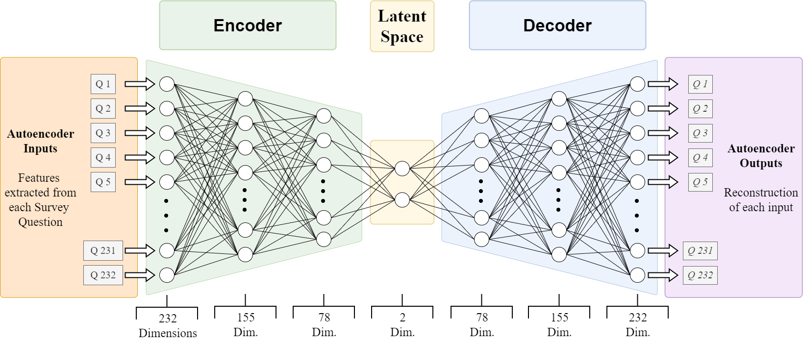
The dataset consisted of responses to survey questions, resulting in 232 features after preprocessing. These features included nominal variables (e.g., categorical choices) and ordinal variables (e.g., ranked scales). The nominal variables were factored out into dummy variables; ordinal variables were all standardized to the same scale using SKLearn OrdinalEncoder.

Encoder and Decoder Design

The autoencoder compresses the 232 input dimensions through three layers: 155, 78, and finally to a 2-dimensional latent space during the encoder stage. The decoder then attempts to reconstruct the original data by reversing these steps using only values in the latent space. Thus, the latent space must compress the original data into a continuous representation that captures complex relationships between input features. This condensed, continuous representation also makes the data more suitable for clustering.

Loss Function

To evaluate how well the autoencoder reconstructed the original input data, we calculate the Reconstruction Loss defined below.

This custome loss function combines binary cross-entropy for nominal variables and Mean Squared Error (MSE) for ordinal variables. Since nominal variables were encoded as binary dummy variables, MSE was inappropriate for them but remained a valid choice for ordinal variables due to their inherent order.

To balance the contributions of the different variable types, I introduced lambda weights to adjust the importance of each component in the loss function:

$ L = \lambda_b \cdot \ell_b + \lambda_o \cdot \ell_o $

Where:

• $ \ell_b $ = binary cross-entropy loss for nominal variables
• $ \ell_o $ = MSE loss for ordinal variables
• $ \lambda_b, \lambda_o $ = weights for respective losses

Since the dataset contained far fewer nominal variables, I reduced their contribution to the loss function to prevent overemphasis while still accounting for their influence. $ \lambda_b $ was set to 0.5 and $ \lambda_o $ set to 1 throughout each experiment to maintain consistency across various autoencoder frameworks.

Activation Functions

I used the ReLU activation function between hidden layers, and the output layer of the decoder employed the Sigmoid function. Ultimately, this combination produced the best results related to the predefined criteria mentioned in the design section above.

Other Autoencoder Parameters

Across the combined and the Pre/Post Covid data splits, each of the following autoencoder parameters remained consistent throughout the project:

• Learning Rate: 0.0001
• Epochs*: 10,000
• Patience*: 20

• Random Seed: 42

  *Note: The model uses an early stopping parameter that halts training once the validation loss stops improving. Additionally, a patience parameter allows training to continue for 20 extra epochs beyond the early stopping point to capture any potential improvements. Although the maximum number of epochs is set to 10,000, this limit was never reached in any training cycle.